Analyze Z7 Smartfin Data
- Decode from base85/ascii85 to human-readable data
- put data in DataFrame for subsequent analysis
- visualize time-series data
- calculate additional wave stats from motion data
In [1]:
import base64
import html
import pandas as pd
import numpy as np
import datetime

from scipy.signal import butter, lfilter, freqz
from scipy import signal
from scipy import integrate
from scipy.signal import find_peaks

import matplotlib.pyplot as plt

import plotly.plotly as py
import plotly.graph_objs as go
from plotly import tools

import pytz
pacific = pytz.timezone('US/Pacific')

from scraping_utils import decoded_to_df

%matplotlib widget
Quick clean-up
- Make sure we don't have hidden, latent variables from a previously executed run
In [2]:
if 'message' in locals():
    del message
if 'messages' in locals():
    del messages

# Only change this to true if the Smartfin's firmware has
# `#define USING_IMU_TEMP_SENSOR 1`
# which is indicative of a faulty TMP116 sensor and an unlikely scenario in future fin distribution
imu_temp_enabled = False
Enter filename
In [3]:
messages = pd.read_csv('Z_Data/Sfin-Z7-00037_190515-000000_CDIP.csv', header=None)
Decode and place data in pandas DataFrame
Only one of decode_particle or decode_google_doc will be used, depending on whether input data come from a single Particle cloud message or an arbitrary number of lines copied out of a Google Sheet and saved in a CSV file.
The CSV file option (decode_google_doc) is far more common.
In [4]:
def decode_particle(message):
    decoded = base64.b85decode(message)
    return decoded

def decode_google_doc(message):
    url_decoded = html.unescape(message)
    decoded = base64.b85decode(url_decoded)
    return decoded
Choose which of above functions to execute in order to get a DataFrame of decoded data
In [5]:
#%% Create DF, decode data, add to DF
# create df
columns = ['type_name', 'time', 'temp', 'wet', 'Ax', 'Ay', 'Az', 'lat', 'lon', 'text', 'batt_v']
df = pd.DataFrame(columns=columns)

if 'message' in locals():
    # decoded = decode_particle(message) # if directly off of Particle (eg CoolTerm readout)
    decoded = decode_google_doc(message) # if getting from Google Doc
    df= decoded_to_df(df, decoded)
elif 'messages' in locals():
    for index, row in messages.iterrows():
        # print(row[1])
        decoded = decode_google_doc(row[1])
        df = decoded_to_df(df, decoded)
else:
    print("Check for proper input variable naming")

df.head()
Out[5]:
Filter based on wetness, good locations, and accelerations, if desired
In [6]:
# obs that are wet and with lat/lon
wet_locations = df[df['wet'] == True]
wet_locations = wet_locations.dropna(subset = ['lat', 'lon'])

# simple_filter = (wet_locations['Ay'] < 1.2) & \
#                 (wet_locations['Ay'] > 0.8)
# wet_locations = wet_locations[simple_filter]
Time-series plots of decoded and wet data
In [9]:
y_var  = 'Ay'

# Create traces
trace1 = go.Scatter(
    x = df['time'],
    y = df[y_var],
    mode = 'markers',
    name = 'all data'
)

trace2 = go.Scatter(
    x = wet_locations['time'],
    y = wet_locations[y_var],
    mode = 'markers',
    name = 'filtered data'
)

data = [trace1, trace2]

# Plot and embed here
py.iplot(data, filename='time-series-scatter')


# plt.plot(, , 'r.', label = 'All data')
# plt.plot(wet_locations['time'], wet_locations[y_var], 'b.', label = 'Filtered data')
# plt.legend()
Out[9]:
Set up filters
In [10]:
#%% Filter out noisy data

# Filter requirements
order = 6
fs = 1       # sample rate, Hz
cutoff = 0.2  # desired cutoff frequency of the filter, Hz

def butter_lowpass(cutoff, fs, order=5):
    nyq = 0.5 * fs
    normal_cutoff = cutoff / nyq
    b, a = butter(order, normal_cutoff, btype='low', analog=False)
    return b, a

def butter_lowpass_filter(data, cutoff, fs, order=5):
    b, a = butter_lowpass(cutoff, fs, order=order)
    y = lfilter(b, a, data)
    return y
Filter and integrate motion sensor data
- Get velocity from integrated accelerations
- Get displacement from integrated velocity
In [40]:
#%% Integrate motion sensor vars

# Get rid of rows where IMU A vals are NaN
motion_df_goodAcc = wet_locations.dropna(subset = ['Ax', 'Ay', 'Az'])

# Covert from G's to m2/s
ax_m2_s = motion_df_goodAcc.loc[:, 'Ax']*9.81
ay_m2_s = motion_df_goodAcc.loc[:, 'Ay']*9.81
az_m2_s = motion_df_goodAcc.loc[:, 'Az']*9.81

# Calculate the magnitude of the 3-D vectors and subtract Earth's gravity
acc_mag = (ax_m2_s**2 + ay_m2_s**2 + az_m2_s**2)**0.5-9.81
#acc_mag = butter_lowpass_filter(acc_mag, 1, 5, 6)

# Integrate acc to get vel
vel_mag = integrate.cumtrapz(acc_mag, dx = 1) # dt = 1 s
vel_mag = np.append(vel_mag, vel_mag[-1])

# Make a Pandas series for math below
vel_series = pd.Series(vel_mag, motion_df_goodAcc.index, name = 'vel (m/s)')
vel_filt = butter_lowpass_filter(vel_series, cutoff, fs, order)
vel_series -= vel_filt
vel_series -= vel_series.mean()

# Integrate vel to get displacement
dis_mag = integrate.cumtrapz(vel_series, dx = 1) # dt = 1 s
dis_mag = np.append(dis_mag, dis_mag[-1])
dis_series = pd.Series(dis_mag, motion_df_goodAcc.index, name = 'displacement (m)')
dis_filt = butter_lowpass_filter(dis_series, cutoff, fs, order)
dis_series -= dis_filt
dis_series -= dis_series.mean()

# Add velocity and displacement back to motion DF
motion_df_integrated = pd.concat([motion_df_goodAcc, vel_series, dis_series], axis = 1)
motion_df_integrated.sort_values(by = 'time', inplace = True)
motion_df_integrated.reset_index(inplace = True, drop = True)

motion_df_integrated.head(20)
Out[40]:
Plot integrated/filtered motion sensor data
In [35]:
#%% Plot Integrals
# fig, axs = plt.subplots(figsize = (8, 6), nrows = 4, sharex = True)

# axs[0].plot(motion_df_integrated['time'], motion_df_integrated.loc[:, 'Ax':'Az'], '.-')
# axs[1].plot(motion_df_integrated['time'], motion_df_integrated.loc[:, 'vel (m/s)'], '.-')
# axs[2].plot(motion_df_integrated['time'], motion_df_integrated.loc[:, 'displacement (m)'], '.-')
# axs[3].plot(motion_df_integrated['time'], motion_df_integrated['temp'], '.')

# axs[0].set_ylabel('G Force (g\'s)')
# axs[1].set_ylabel('Vel (m/s)')
# axs[2].set_ylabel('Disp (m/s)')
# axs[3].set_ylabel('Temp $^o$F')
# axs[3].set_xlabel('Time (s)')
# fig.autofmt_xdate()
# date_format = '%H:%M:%S'
# myFmt = mdates.DateFormatter(date_format, tz = pacific)
# axs[2].xaxis.set_major_formatter(myFmt)

# plt.tight_layout()

# Create traces
trace1 = go.Scatter(
    x = motion_df_integrated['time'],
    y = motion_df_integrated['Ax'],
    mode = 'lines+markers',
    name = 'Ax'
)

trace2 = go.Scatter(
    x = motion_df_integrated['time'],
    y = motion_df_integrated['Ay'],
    mode = 'lines+markers',
    name = 'Ay'
)

trace3 = go.Scatter(
    x = motion_df_integrated['time'],
    y = motion_df_integrated['Az'],
    mode = 'lines+markers',
    name = 'Az'
)

trace4 = go.Scatter(
    x = motion_df_integrated['time'],
    y = motion_df_integrated['vel (m/s)'],
    mode = 'lines+markers'
)

trace5 = go.Scatter(
    x = motion_df_integrated['time'],
    y = motion_df_integrated['displacement (m)'],
    mode = 'lines+markers'
)

trace6 = go.Scatter(
    x = motion_df_integrated['time'],
    y = motion_df_integrated['temp'],
    mode = 'lines+markers'
)

# data = [trace1, trace2]

fig = tools.make_subplots(rows = 4, cols = 1, shared_xaxes=True)

fig.append_trace(trace1, 1, 1)
fig.append_trace(trace2, 1, 1)
fig.append_trace(trace3, 1, 1)
fig.append_trace(trace4, 2, 1)
fig.append_trace(trace5, 3, 1)
fig.append_trace(trace6, 4, 1)


# Plot and embed here
py.iplot(fig, filename='all-integrated')
Out[35]:
Find peaks in displacement signal, $\eta$
- repeat for the negative signal to find troughs
In [36]:
eta_plus = motion_df_integrated['displacement (m)']
eta_minus = -1*motion_df_integrated['displacement (m)']
time = motion_df_integrated['time']

peaks, _ = find_peaks(eta_plus, distance = 3)
troughs, _ = find_peaks(eta_minus, distance = 3)
In [37]:
trace1 = go.Scatter(
    x = time,
    y = eta_plus,
    mode = 'lines+markers',
    name = 'Free Surface'
)

trace2 = go.Scatter(
    x = time[peaks],
    y = eta_plus[peaks],
    mode = 'markers',
    marker = dict(
        size = 8,
        color = 'rgb(255,0,0)',
        symbol = 'cross'
    ),
    name = 'Detected Peaks'
)

trace3 = go.Scatter(
    x = time[troughs],
    y = eta_plus[troughs],
    mode = 'markers',
    marker = dict(
        size = 8,
        color = 'rgb(255,0,255)',
        symbol = 'cross'
    ),
    name = 'Detected Troughs'
)

fig = tools.make_subplots(rows = 1, cols = 1, shared_xaxes=True)

fig.append_trace(trace1, 1, 1)
fig.append_trace(trace2, 1, 1)
fig.append_trace(trace3, 1, 1)

# Plot and embed here
py.iplot(fig, filename='peaks')
Out[37]:
In [38]:
print(len(peaks), len(troughs))
Calculate amplitude and $H_s$
In [39]:
# Calculate shorter array of peaks vs. troughs and make sure both arrays are same size
n_peaks = len(peaks)
n_troughs = len(troughs)
n_lesser = np.min([n_peaks, n_troughs])

# Grab heights of peaks and troughs up to length of smaller array
h_peaks = eta_plus[peaks].values[:n_lesser]
h_troughs = eta_plus[troughs].values[:n_lesser]

# Calculate height as peak minus trough (amplitude x 2)
height = np.abs(h_peaks-h_troughs)

# Calculate length of top third of all waves observed
n_topthird = int(len(height)/3)

# Calculate height of top third of all waves
h_topthird = (height[np.argsort(height)[-n_topthird:]])
# print(h_topthird)

# Calculate significant wave height: mean of height of top third
h_s = np.nanmean(h_topthird)
print("Significant wave height:", h_s, "m")
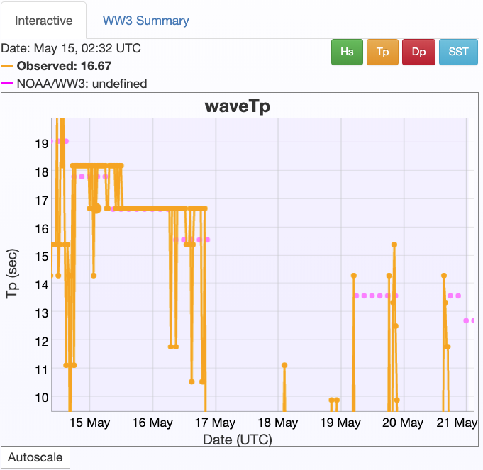
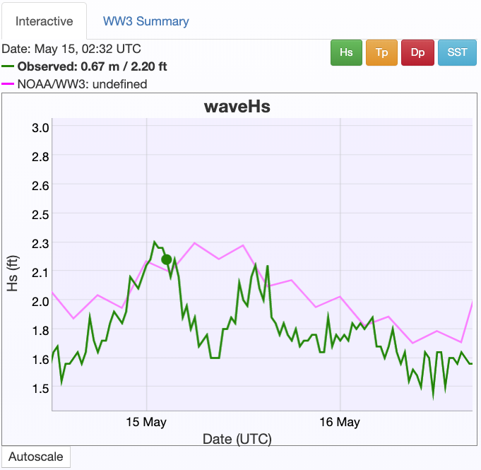
CDIP Comparison
At the same time as these data were collected, here is what was being recorded by the nearby CDIP Wave Rider buoy
significant wave height (about an order of magnitude smaller than my clearly erroneous calculation above):
and peak period: