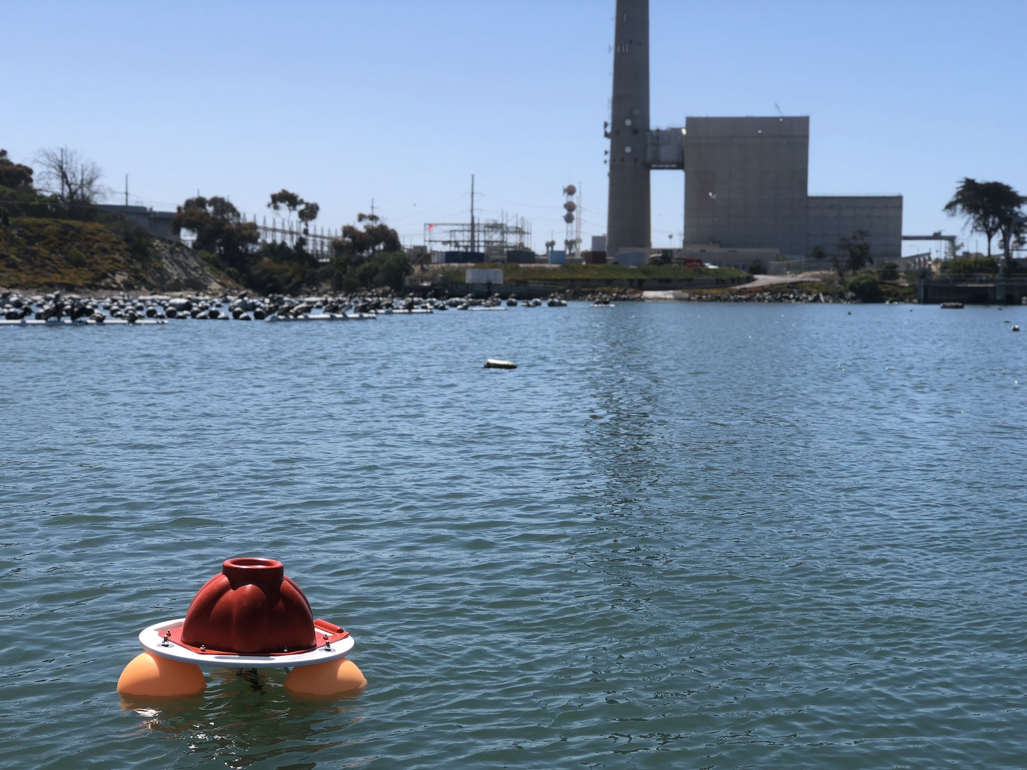
Carlsbad Aquafarm SeapHOx
I am posting this not as an example of active research, but instead as an example of an open Jupyter notebook which I used to conduct a preliminary analysis. I’m no longer actively maintaining this analysis (though the sensor is still deployed as part of a SCCOOS grant), but leaving this page up to show how we conduct some of our real-time data communications and analysis.
The following is a Jupyter notebook with a Python script that I’ve been using occasionally to scrape a Google Sheet with near-real-time data. The Google Sheet updates ~ 2x/hr but this website is static so it updates only when I manually do so. See my ThingSpeak channel for the near-real-time data output.
Google Sheets Scraper
Goal: scrape the Google Sheet with autofilling data from the Particle Electron at Carlsbad Aquafarm Google Sheet named "SeapHOx_OuterLagoon" is here
import numpy as np
import pandas as pd
# import seaborn as sns
import matplotlib.pyplot as plt
import matplotlib.ticker as ticker
import datasheets
import os

%matplotlib inline
Scrape Google Sheets
Use datasheets library, following directions from https://datasheets.readthedocs.io/en/latest/index.html
client = datasheets.Client()
workbook = client.fetch_workbook('SeapHOx_OuterLagoon')
tab = workbook.fetch_tab('Sheet1')
electron_array = tab.fetch_data()
electron_array.head()
Get SeapHOx String, Parse, Remove Bad Transmissions
data_col = electron_array.iloc[:, 1]
data_array = pd.DataFrame(data_col.str.split(',', expand = True))

# Get rid of rows that don't start with "20" as in "2018"; this is foolproof until 2100 or 20 shows up elsewhere in a bad row, I guess
good_rows = (data_array.iloc[:, 0]).str.contains('20')
good_rows.fillna(False, inplace = True)
data_array = data_array[good_rows]
Rename and Reindex
data_array.columns = ['Date', 'Time', 'V_batt', 'V_int', 'V_ext', 'P_dbar', 'pH_int', 'O2_uM', 'temp_SBE', 'sal_SBE', 'V_batt_elec', 'charge_status']
data_array.set_index(pd.to_datetime(data_array['Date'] + ' ' + data_array['Time']), inplace = True)
data_array.drop(['Date', 'Time'], axis = 1, inplace = True)
data_array.head()
Filter
- Filter based on date
- Cast to type float (for some reason the str.split leaves it as arbitrary object)
- This was necessary in early notebook as the input data wasn't filtered at all but the Google Sheet should be cleaner to begin with (i.e., no land data)
- Filtration may come in handy later so keep this here for now
date_filt = data_array.index > '2017-09-07 18:30:00'
data_filt = data_array[date_filt]

import pytz
pacific = pytz.timezone('US/Pacific')
data_filt.index = data_filt.index.tz_localize(pytz.utc).tz_convert(pacific)

data_filt = data_filt.astype('float')

data_filt.tail()
# data_filt.V_press
Set manual limits
- manually set reasonable limits
- todo: implement other QARTOD standards for range tests, spike tests, noise tests, rate of change tests, etc.
pH_int_min = 7.5
O2_uM_max = 400

data_filt.O2_uM[data_filt.O2_uM > O2_uM_max] = np.nan
data_filt.pH_int[data_filt.pH_int < pH_int_min] = np.nan
Plot
fig, axs = plt.subplots(6, 1, figsize = (10, 10), sharex = True)
axs[0].plot(data_filt.index, data_filt.V_batt)
axs[0].set_ylabel('V_batt')
ax2 = axs[0].twinx()
ax2.plot(data_filt.index, data_filt.V_batt_elec, 'r')
ax2.set_ylabel('V_batt_elec', color='r')
ax2.tick_params('y', colors='r')

axs[1].plot(data_filt.index, data_filt.P_dbar)
axs[1].set_ylabel('P (dbar)')

axs[2].plot(data_filt.index, data_filt.sal_SBE)
axs[2].set_ylabel('Salinity')

axs[3].plot(data_filt.index, data_filt.temp_SBE)
axs[3].set_ylabel('Temp (C)')

axs[4].plot(data_filt.index, data_filt.V_int)
axs[4].set_ylabel('V_int')
ax2 = axs[4].twinx()
ax2.plot(data_filt.index, data_filt.V_ext, 'r')
ax2.set_ylabel('V_ext', color='r')
ax2.tick_params('y', colors='r')

axs[5].plot(data_filt.index, data_filt.pH_int)
axs[5].set_ylabel('pH')
ax2 = axs[5].twinx()
ax2.plot(data_filt.index, data_filt.O2_uM, 'r')
ax2.set_ylabel('O2 (uM)', color='r')
# ax2.set_ylim([0, 400])
ax2.tick_params('y', colors='r')

axs[0].xaxis_date() # make sure it knows that x is a date/time

for axi in axs.flat:
#     axi.xaxis.set_major_locator(plt.MaxNLocator(3))
#     print(axi)
    axi.yaxis.set_major_locator(plt.MaxNLocator(3))
#     axi.yaxis.set_major_formatter(ticker.FormatStrFormatter("%.02f"))

fig.autofmt_xdate() # makes the date labels easier to read.
plt.tight_layout()
plt.savefig('test_dep_01.png')

fig, axs = plt.subplots(1, 1, figsize = (10, 10), sharex = True)
pHOx = axs.scatter(x = data_filt.pH_int,
                   y = data_filt.O2_uM,
                   c = data_filt.P_dbar,
                   s = 100)
axs.set_xlabel('pH (int)')
axs.set_ylabel('O2 (uM)')
plt.colorbar(pHOx, label = 'P (dbar)');

cmap = plt.get_cmap('coolwarm')
corr = data_filt.corr()
corr.style.background_gradient(cmap, axis=1)\
    .set_properties(**{'max-width': '80px', 'font-size': '10pt'})\
    .set_caption("SeapHOx Correlations")\
    .set_precision(2)